Model Run Options

For model run options, specify the duration of the run period in the Start_Year and End_Year variables. Set the model warm up period in the Warm_Up_Period variable, as shown in Figure 5. You can get results in Comma Separated Values (CSV) format by setting the Print_CSV option to 1, else, set it to 0.

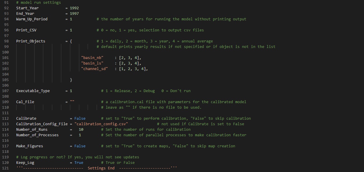
Figure 5: Model run and calibration settings section

You have the option to run the model after setup using the Release or Debug executables by setting Executable_Type to 1 or 2 respectively. Set it to 0 to setup the model without running it.

You can set the model to give results at specific timesteps using the Print_Objects variable. Set the name of the output variables you want to specify and the list of the results timesteps needed as demonstrated in Figure 5. Include 1, 2, 3 and 4 to print daily, monthly, yearly and annual average results respectively. The variables available for selection are listed as follows:

basin_wb, basin_nb, basin_ls, basin_pw, basin_aqu, basin_res, basin_cha, basin_sd_cha, basin_psc, region_wb, region_nb, region_ls, region_pw, region_aqu, region_res, region_cha, region_sd_cha, region_psc, lsunit_wb, lsunit_nb, lsunit_ls, lsunit_pw, hru_wb, hru_nb, hru_ls, hru_pw, hru-lte_wb, hru-lte_nb, hru-lte_ls, hru-lte_pw, channel, channel_sd, aquifer, reservoir, recall, hyd, ru, pest.

For more information on this variables, see the SWAT+ Input Output Documentation (Click here to view).

Calibration

If you want to apply parameters to the model after setup, specify the name of the parameter file in the Cal_File variable; leave “” if you do not want to apply parameters. Remember to have the parameter file in the calibration folder under data.

You can perform calibration on the model if you already know the outlet number that will need to be calibrated. Information on the calibration such as observation file name, parameter names and ranges are all set in a separate CSV file placed in the calibration directory. The name of this configuration file should be placed on the Calibration_Config_File.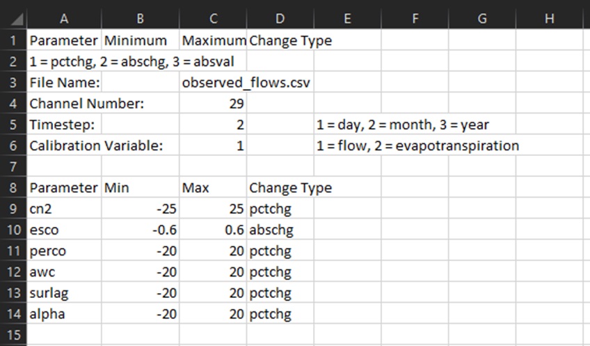

Figure 6: Example of Calibration_Config_File

Calibration_Config_File looks. It is important to know that the calibration is solely done by trying out parameter sets generated by lating hypercube sampling and chosing the parameter set that gives the highest Nash-Sutcliffe Efficiency Value. The Number_of_Processes variables allows you to perform the calibration using parallel processing which speeds up the calibration by trying multiple parameter sets at a time.